Segmenting with R
Segmenting all WAVE files in a directory #
The first method of segmenting files in R we will discuss is the
split_sound_files function provided by the warbleR package. You would
typically use this function if you need to segment your files based on either
duration, or number of segments to create per file. Since acoustic indices are
typically calculated on 60 second segments of audio, you could use this
function to split long files into 60 second segments, or else whatever length
you desire. See the function documentation
here
The example code below will look for sound files in the data folder of your
current R working directory. For these first examples, the data folder
contains a single WAVE file (CC1_20171010_125500.wav), which has a duration
of just over 1 minute. You can download the practice WAVE file
here
As mentioned, the split_sound_files function can segment your WAVE files
into specific durations, or into a specific number of segments. In this first
example, the code below will segment our WAVE file by a specified
duration, into 15 second segments:
library(warbleR)
split_sound_files(path = "data", sgmt.dur = 15, pb = TRUE)
##          org.sound.files               sound.files start      end
## 1 CC1_20171010_125500.wav CC1_20171010_125500-1.wav     0 15.00000
## 2 CC1_20171010_125500.wav CC1_20171010_125500-2.wav    15 30.00000
## 3 CC1_20171010_125500.wav CC1_20171010_125500-3.wav    30 45.00000
## 4 CC1_20171010_125500.wav CC1_20171010_125500-4.wav    45 60.00000
## 5 CC1_20171010_125500.wav CC1_20171010_125500-5.wav    60 60.00036
Because the input file was slightly greater than 60 seconds, a fifth WAVE file
was generated, with a duration of 0.00036 seconds.
Instead of specifying the duration, in this next example we will specify the number of segments. The example code below will segment the file into four evenly sized segments:
library(warbleR)
split_sound_files(path = "data", sgmts = 4, pb = TRUE)
##          org.sound.files               sound.files    start      end
## 1 CC1_20171010_125500.wav CC1_20171010_125500-1.wav  0.00000 15.00009
## 2 CC1_20171010_125500.wav CC1_20171010_125500-2.wav 15.00009 30.00018
## 3 CC1_20171010_125500.wav CC1_20171010_125500-3.wav 30.00018 45.00027
## 4 CC1_20171010_125500.wav CC1_20171010_125500-4.wav 45.00027 60.00036
In both cases, our data directory now contains our original WAVE file, as
well as the newly generated segments.
Specific segmentation of an audio file #
Sometimes you may want to import or extract a specific segment of a recording, rather than segment all of your audio files. There are two main approaches we can take to do that in R.
The first approach is to directly import a specific segment of a WAVE
file, when using the tuneR readWave function, or when using the wrapper
function read_sound_file from the warbleR package. If you already know which
section of a file you would like to work with, this saves you from first
importing a full length file, and then creating a segment.
In the example below, our practice file (CC1_20171010_125500.wav) is imported,
but only the audio between 10 and 20 seconds, instead of the full 60 second
file. The actual WAVE file will not be modified.
library(tuneR)
CC1_20171010_125500_10_20 <-
        readWave(
                filename = "data/CC1_20171010_125500.wav",
                from = 10,
                to = 20,
                units = "seconds")

CC1_20171010_125500_10_20
## Wave Object
##	Number of Samples:      220500
##	Duration (seconds):     10
##	Samplingrate (Hertz):   22050
##	Channels (Mono/Stereo): Mono
##	PCM (integer format):   TRUE
##	Bit (8/16/24/32/64):    16
library(warbleR)
CC1_20171010_125500_10_20 <-
        read_sound_file(
                X = "data-segmenting/CC1_20171010_125500.wav",
                from = 10,
                to = 20)

CC1_20171010_125500_10_20
## Wave Object
##	Number of Samples:      220500
##	Duration (seconds):     10
##	Samplingrate (Hertz):   22050
##	Channels (Mono/Stereo): Mono
##	PCM (integer format):   TRUE
##	Bit (8/16/24/32/64):    16
The second approach is to extract a specific segment from an existing Wave
object in R, using the extractWave function. In the following example, we will
extract just the audio from 2 to 8 seconds, from the Wave object we imported
in the previous example (CC1_20171010_125500_10_20). We will store the output
in a new object.
library(tuneR)
CC1_20171010_125500_10_20_extract <-
        extractWave(
                CC1_20171010_125500_10_20,
                from = 2,
                to = 8,
                xunit = "time")
Inspecting the new object we created (CC1_20171010_125500_10_20_extract) shows
a duration of 6 seconds, instead of the original 10 seconds.
CC1_20171010_125500_10_20_extract
## Wave Object
##	Number of Samples:      132301
##	Duration (seconds):     6
##	Samplingrate (Hertz):   22050
##	Channels (Mono/Stereo): Mono
##	PCM (integer format):   TRUE
##	Bit (8/16/24/32/64):    16
Hint:
Remember, you can use thewriteWavefunction at any time on aWaveobject to store the output as aWAVEaudio file. Try savingCC1_20171010_125500_10_20_extractas aWAVEfile.
Specific segmentation of all audio files in a directory #
Sometimes when importing audio files, you may wish to import just a specific
time segment for each file in a directory. For example, if your audio files
consistently contained interference at the start and end of each recording, you
might like to ignore the first and last 5 seconds of each recording. In this
case, we can deal with this directly when importing our files into R, without
having to modify the WAVE files on the disk, by using the to and from
arguments in the readWave function. For the purposes of this example, our
data directory now contains three copies of our practice WAVE file.
We start by creating a list of all the WAVE files in our data directory:
files <-
        list.files(path = "data",
                   pattern = "\\.wav$",
                   full.names = TRUE)
Checking the contents of our object files shows it contains the names of our
three audio files:
files
[1] "data/CC1_20171010_125500_1.wav"
[2] "data/CC1_20171010_125500_2.wav"
[3] "data/CC1_20171010_125500_3.wav"
Next, we use the lapply function to apply the readWave function to each of
our files. In this example, we pass additional arguments from and to, to
specify the section of each file to be imported. Therefore, only the audio
between 5 and 55 seconds of each file will be imported. To import the full
duration audio files just use lapply(files, readWave).
waves_list <-
        lapply(files,
               readWave,
               from = 5,
               to = 55,
               units = "seconds")

# adds names to each element of the list based on file name
names(waves_list) <- gsub(".*\\/","", files)
We have now imported our three audio files, which are stored as Wave objects
within a list called waves_list. Lets take a look at a spectrogram of the
first list element (i.e. the first audio file):
library(seewave)
spectro(waves_list[[1]], main = names(waves_list)[1], fastdisp = TRUE)
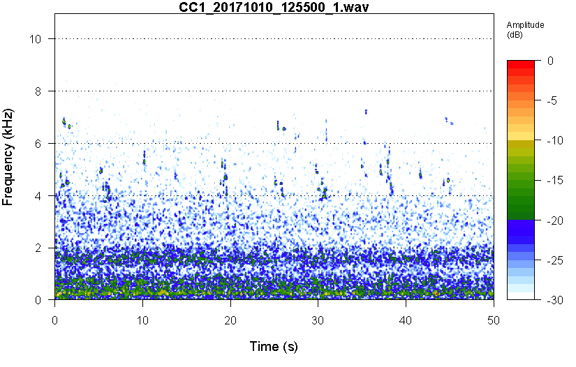
Success! Our WAVE files have been imported, without the first and last 5 seconds
of audio, and are stored as Wave objects ready for analysis. Try running the
above code with 2 instead of 1 to see the spectrogram for the second audio
file.