Harnessing acoustic data and Generalised Dissimilarity Modelling to examine compositional turnover of avian species.
Developed in a collaboration between Open Ecoacoustics & EcoCommons.
Summary #
Understanding changes in species composition across temporal and spatial scales can provide important insights for management and conservation of biodiversity, particularly with increasing threats due to climate change and land clearing. Traditionally, species community surveys, performed with consistent methodology, are used to model compositional dissimilarity. However, the aim of this project was to demonstrate how data collected by passive acoustic monitoring (PAM) may also be used to examine spatial variation in species composition across a landscape.
This case study uses annotated acoustic data from a previously published study
(Doohan et al. 2019
The R code used to generate these results is provided.
Introduction #
Faunal biodiversity is known to be influenced by vegetation condition, structure and diversity. Given the history and extent of vegetation clearing across Australia, it is essential that the relationships between vegetation and faunal biodiversity are understood. The Mulga Lands bioregion, which stretches from south western Queensland into northern New South Wales, is one such area that has experienced high levels of vegetation clearance. This region provides a unique habitat for many arid, semi-arid and temperate species. However, the effects of regrowth vegetation on community composition is poorly understood, particularly in semi-arid and arid environments. Birds are often sensitive to the effects of landscape modification and clearing, and therefore represent good candidate species to study the effects of regrowth vegetation. As a result, avian biodiversity was examined in the Mulga Lands bioregion, in relation to various stages of vegetation growth.
This research involved the use of passive acoustic monitoring devices, which can
capture large scale datasets on environmental soundscapes. Analysis of those
soundscapes represents the focus of the emerging field of ecoacoustics. The
increasing use of passive acoustic monitoring represents an ever-growing body of
data which can be harnessed to answer an array of ecological questions (e.g.
A2O
Methods #
The data used in this case study consisted of avian species identifications from
acoustic recordings obtained from a previous study undertaken by Doohan et al.
(2019). Their study took place in the Bowra Wildlife Sanctuary, an Australian
Wildlife Conservancy property approximately 850km west of Brisbane, Australia.
The data came from nine study sites in total, which were classified based on
their time since clearing occurred, representing three regrowth sites (cleared
within the last 15 years; site code NR), three intermediate regrowth sites
(cleared between 15 and 30 years; site code IR) and three old growth sites (no
clearing events within the last 30 years; site code OG and OM) (Figure 1). One
acoustic monitoring device was deployed at each site (model SM3; Wildlife
Acoustics), and set to record the dawn chorus each day continuously for 3 hours
(recorded as WAV format, in mono at a sample rate of 22,050 Hz) during the
study period of 28 days (29th August 2017 – 25th September 2017). From this
data, 45 hours of audio were processed by Doohan et al. (2019)
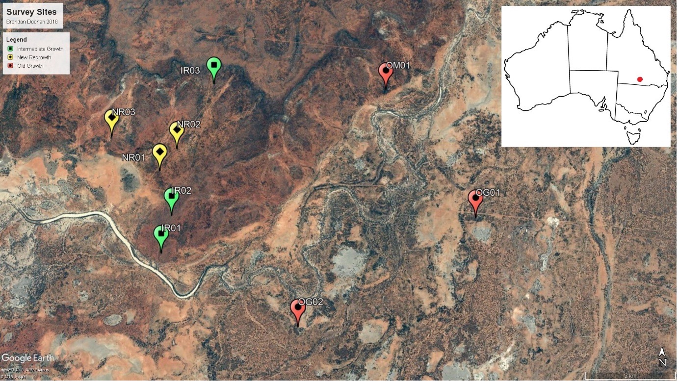
Figure 1: Study site locations represented by pins (yellow: new regrowth, green: intermediate regrowth, red: old growth). Inset map of Australia indicates location of the study area.
For the current project, we demonstrate how an existing annotated acoustic dataset, along with study site environmental data, can be used to model compositional dissimilarity of avian species in relation to various environmental predictors. Therefore, a generalised dissimilarity model (GDM) approach was chosen. The benefit of this method is that it can statistically relate beta diversity to environmental gradients, while accounting for two important nonlinearities present in more traditional ecological methods (see Ferrier et al., 2007).
Using the GDM package in R (function: GDM with default parameters), a model was
fit using a range of environmental variables that were collected in the field at
the location of each acoustic sensor. Vegetation assessments were undertaken by
Doohan et al. (2019)
The final variables included in the model were:
- Tree height (m)
- Tree cover (%)
- Diameter at breast height (DBH, cm)
- Shrub height (m)
- Distance to nearest water course (QLD Waterways spatial dataset, m)
- Geographic distance (between sites, m)
A model using raster layer Soil Adjusted Vegetation Index (SAVI) from Sentinel Hub was also performed, but discontinued due to its low explanatory power (percent deviance explained = 2.001).
Results #
The model had a percent deviance explained of 27.159, representing the variation in observed dissimilarities explained by the model. A slight positive linear relationship was seen, whereby as the predicted ecological distance between sites increased (predictors), so too did observed compositional dissimilarity (Figure 2). Of the environmental predictors, the sum of I-spline coefficients was highest for the predictor value tree cover, indicating the greatest effect on compositional dissimilarity. It was seen by the gradient of the slope that changes between 0 to 30% tree cover resulted in the greatest changes in predicted dissimilarity between study site pairs (Figure 2). However, a permutation assessment showed that the model was not statistically significant (p = 0.370). The intercept of the model was 0.206, which represents the expected dissimilarity between sites when the environmental predictors are equal.
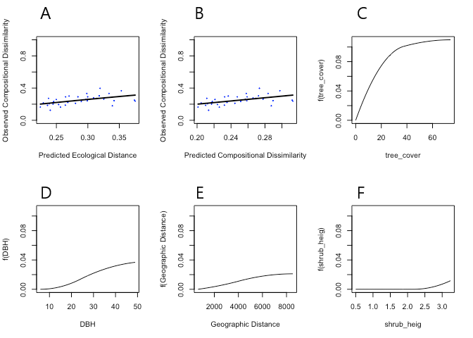
Figure 2: Main output plots of the GDM. A: observed compositional dissimilarity as a function of predicted ecological distance, where each point represents a site pair, and the line represents the GDM-predicted dissimilarity. B: Observed compositional dissimilarity as a function of predicted compositional dissimilarity, where the line represents a line of equality. C – F: Plotted GDM spline functions for each environmental predictor variable.
Discussion #
These results successfully demonstrate a simple workflow in which acoustic datasets can be leveraged to provide insight into patterns of biodiversity change relative to environmental predictors. In this case, the original sampling design could have limited the model’s ability to predict changes in composition throughout the landscape relative to the environmental predictors. For example, all sensors were located inside a patch of vegetation at least 150 m or greater in diameter. The total number of sample sites was also small, and sensors were positioned across a relatively small spatial. Nevertheless, this is a great example workflow of how annotated acoustic data can be used to perform more robust modelling methods, such as GDM.
In this example, study site vegetation survey data was available at the location of each recorder. However, it is also possible to use spatially complete gridded environmental data with the GDM package, such as remotely sensed data in raster format. This allows projection of the model across the spatial grid, to map predicted patterns of dissimilarity.
With the growing body of acoustic data, coupled with remotely sensed data or ground-survey metadata, it will be possible to examine patterns of biodiversity variation across large spatial and temporal scales. Identifying environmental factors that are important drivers for species occurrences can help to guide land management, landscape rehabilitation and inform restoration guidelines. It is also possible to make predictions about compositional turnover related to changes in environmental conditions, such as land cover, or temperature (climate change).
Acknowledgements #
- I would like to first acknowledge the authors of the original publication from
which this data was sourced: Brendan Doohan, Jeanette Kemp, and Susan Fuller.
The article was published Global Ecology and Conservation (2019), and is
available here
. - This project was internally funded by the Queensland University of Technology.
- We thank the Australian Wildlife Conservancy for site access, previous species records and facilitation of the project.
- Prof. Paul Roe for the loan of additional sensors.
- The Ecosounds platform
, for management, access, visualisation, and analysis of the acoustic data used in this project.
- The EcoCommons
platform: - Read more about ecoacoustic integration with EcoCommons here
. - See the new community modelling (GDM) R package
by EcoCommons. - Visit the Educational Material
section to learn more about the platform.
- Read more about ecoacoustic integration with EcoCommons here