The Australian Acoustic Observatory, Hoot Detective, & the impact of good data on Species Distribution Models
By Dr Andrew Schwenke
Developed in a collaboration between Open EcoAcoustics & EcoCommons.
Introduction #
The Australian Acoustic Observatory (A2O) is a continental-scale acoustic sensor
network that provides data for hundreds of acoustic sensors across seven
Australian ecoregions. This data is freely available to researchers, citizen
scientists, and the general public, for use under CC BY 4.0
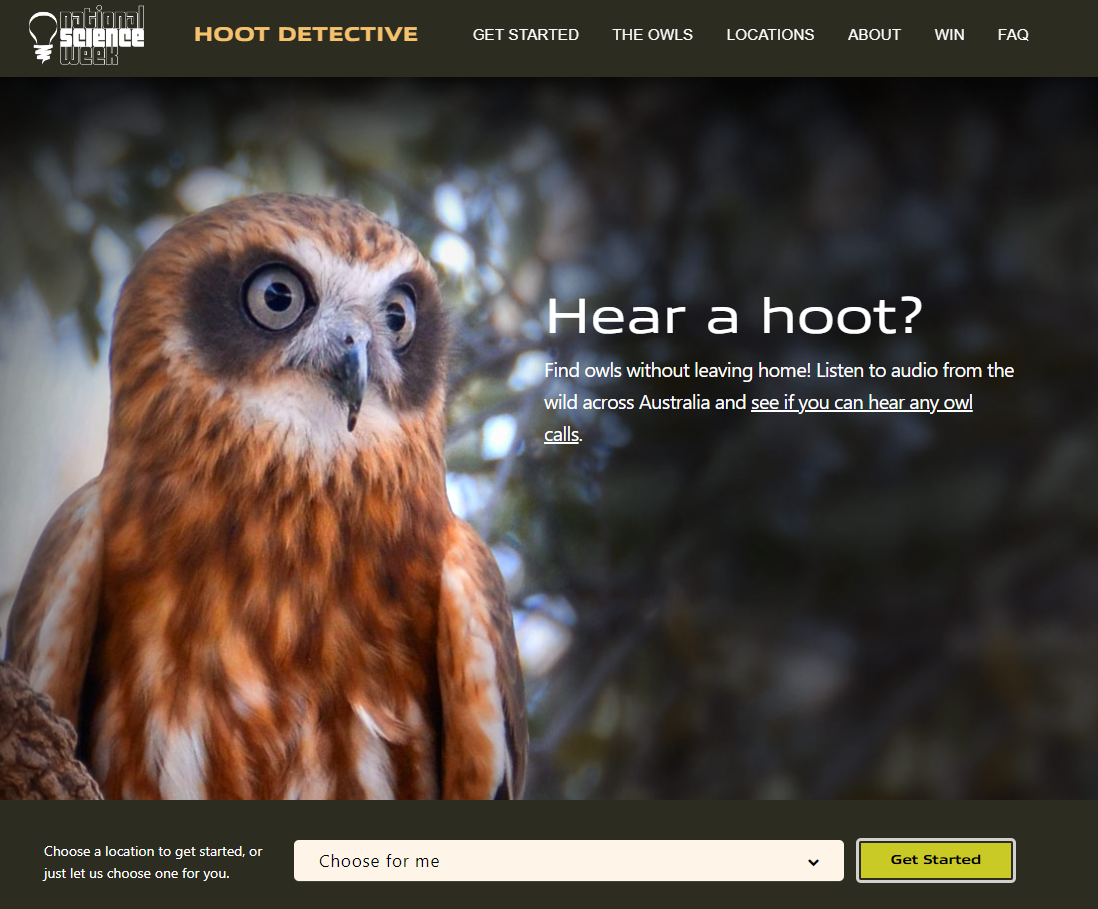
Figure 1: Hoot Detective website.
First, occurrence data for most fauna in Australia are not systematically collected at geographic scales. Most data for species that vocalise are highly biased with the most sampling done near the handful of urban areas in what is otherwise the remote continent of Australia. Dealing with sampling bias in species distribution modelling is one of the biggest challenges to generating optimal results. However, these sampling issues can be virtually eliminated by deploying ecoacoustic sensors based on sampling protocols that are representative of both geographic and environmental space. The Australian Acoustic Observatory achieves this at a continental scale, with around 360 continuously operating acoustic sensors deployed across Australia in a variety of unique ecosystems.
Second, while there will always be variation in detection probability in any fauna survey, ecoacoustic data takes a huge leap toward delivering standardised data. In species distribution modelling, the complications arising from variable detection rates have led many researchers to model detection, using something called occupancy modelling. Indeed, occupancy modelling may be helpful when accounting for variable detection rates between sites and sensors when working with acoustic data. But when using acoustic sensors, survey effort is much more standardised than in human observation data, which can reduce or eliminate the need to use such techniques. Furthermore, species identifications from ecoacoustic data are verifiable and can exist as a persistent record for future use and evaluation.
Third, the field of species distribution modelling has thousands of papers related to using presence only modelling methods, or using binomial methods (presence / absence) with pseudo-absence data. Pseudo absence data attempts to make the best possible guess as to where species might be absent or at the least ensures that random pseudo-absence points are not selected in areas where there is zero chance that the species might be present. As acoustic sensors are increasingly deployed an understanding of detection probability begins to emerge for different sensors and different species. In other words, we can determine how long a sensor should be left out before we are nearly certain that the species of interest is not present. Once a sensor is left out the required amount of time, a true absence location is generated, and such data have significant impacts on how well you can model species distributions using a variety of both statistical and machine learning techniques.
Fourth, an acoustic device records every single call a species makes near a monitor. While human observation data can also provide such data, it would be a massive undertaking to deliver that kind of data at scale. Yet, for many species that vocalise, one can expect call rates to be highest in areas and times of year when species are breeding, and vocalisation rates may even be higher in areas of higher quality habitat (at least for some species). Modelling the distribution of call frequency or abundance has been done far less in the literature than presence only modelling, yet the potential insights from such models are clear. For select species, an area with more calling might be more important for the species, and an area with more individuals calling might be relatively more important than the more silent areas.
The advantages and assumptions discussed so far are likely to vary depending on the specific research question and species of interest. Nevertheless, the purpose of this use case is to demonstrate the kinds of results that can be generated with presence absence vs presence only data, and the insights that could be gained from predicting the spatial variation in call frequency. We argue the benefits are clear, and ask you to help deliver this kind of data at scale.
Methods #
The data were obtained from the historical Hoot Detective project, and consisted
of annotations for five owl species: Masked Owl (Tyto novaehollandiae), Eastern
Barn Owl (Tyto javanica), Barking Owl (Ninox connivens), Powerful Owl (Ninox
strenua), and Southern Boobook (Ninox boobook). All data, including audio
recordings, annotations, and associated sensor metadata, is available for
download and use from the A2O data portal
Data preparation #
The Hoot Detective project resulted in 28723 segments of annotated audio, from 37 sensors. Each segment of audio was 10 seconds in length, resulting in a total of just under 80 hours of annotated audio. Audio segments came from most days spanning between June, 2019, until July, 2021 (Figure 2). These annotations were summarised in R to get occurrence data for each species, which included determining if at any point the target species was recorded (presence) or was absent from recordings (absence).
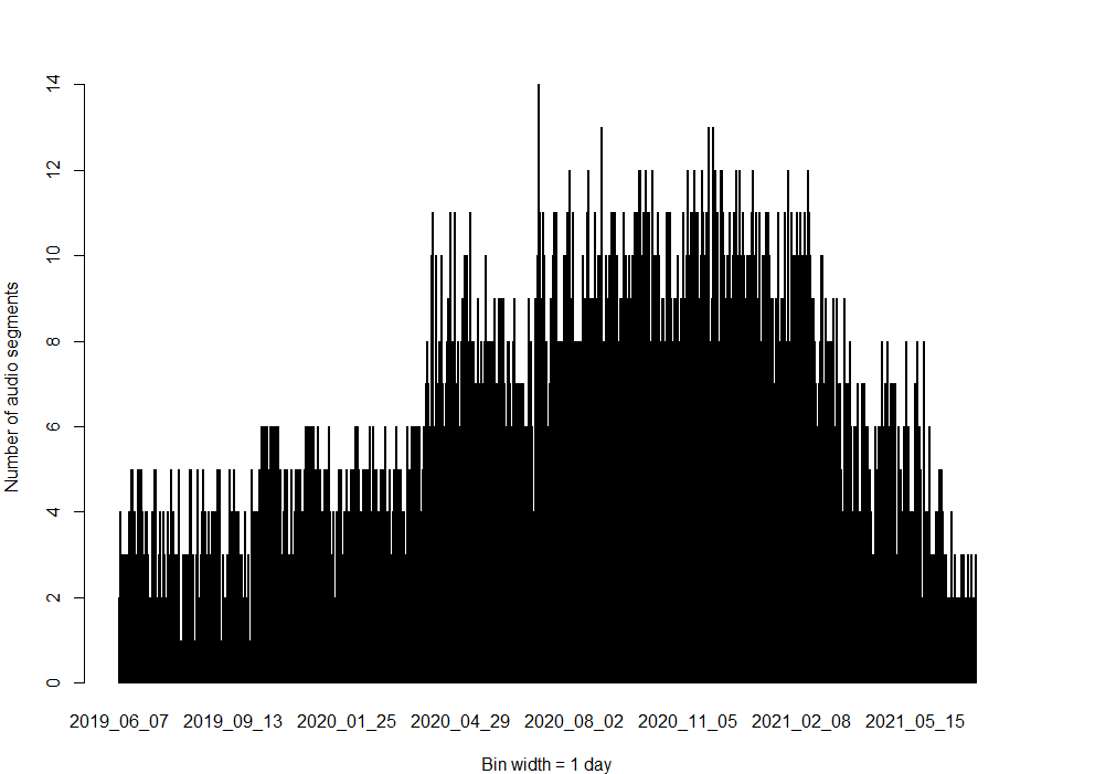
Figure 2: Histogram demonstrating total frequency of annotated audio segments per day in the Hoot Detective data set.
A Powerful Owl presence was recorded in Western Australia, which is quite far outside of the recognised distribution. Therefore, Powerful Owl records were filtered further, using a buffered boundary of the known distribution extent derived from ALA records, to remove these potentially anomalous records.
The A2O uses a paired sensor design, with four sensors per site. The distance between sensors is typically within 500m to 5000m. Therefore, we first attempted to use environmental layers at a high spatial resolution (25m), to capture fine scale variation between proximate sensors.This came at a high computer processing cost. Even working with buffered extents, and using a high-performance PC, the process was slow, highlighting the challenges of using such high resolution data. As a result, we decided to instead use a 250m resolution for preliminary analyses in R, and a 1000m resolution on the ecocommons platform. To get a raster stack for the extent of Australia, the terra package in R was used to crop and mask layers to a vector of the Australian boundary. Layers were then resampled from their original resolution where necessary to 250m, using bilinear interpolation for continuous bioclim data, mean for forest canopy and height, and nearest neighbour for categorical data. All layers were projected to the project CRS (EPSG: 4326). For Powerful Owl, the raster stack was cropped and masked to the buffered boundary extent representing the known distribution.
Analysis #
Powerful Owl presence data were used to extract environmental variable values
from eastern Australia, and the resulting presence data and environmental
rasters were used in a Maxent model in R (see example code)
Presence only vs presence absence comparisons were made within the EcoCommons platform. Evironmental predictors were at 1 km resolution and included the ANU Bioclim variables, 5,6,13 & 17, run in BioClim and SRE for presence only, and ANN, RF, & MARS. First, the presence only occurrence records were used to generate a BioClim model prediction using default settings. Then the presence absence data were used in an Artificial Neural Network (ANN) model, Random Forest model, and multivariate adaptive regression splines (MARS).
To examine the potential of predicting call frequency across Australia we
selected the Southern Boobook which was recorded at all but one station (mean
137 vocalisations, range 0 to 993). We then extracted raster grid values from
the two forest area variables, bioclim variables 5,6 and 17, and NVIS, a
national vegetation classification. We then ran a Boosted regression tree (BRT)
model specifying a Poisson distribution (see example code)
Results #
The 37 monitoring stations that were included in the Hoot Detective project are spread across large areas of Australia, so it is perhaps not surprising that data availability and results varied between species. For example, the Powerful Owl which is only found in eastern Australia had relatively few locations where they were recorded. Chance resulted in more detections of Powerful Owl in southeast Queensland in observatory data, and that bias is reflected in attempts with multiple methods to predict their distribution using only observatory data. Nonetheless, the presence-only model MaxEnt proved to be the best at approaching predictions of the actual distribution of Powerful Owl in eastern Australia (Figure 3).
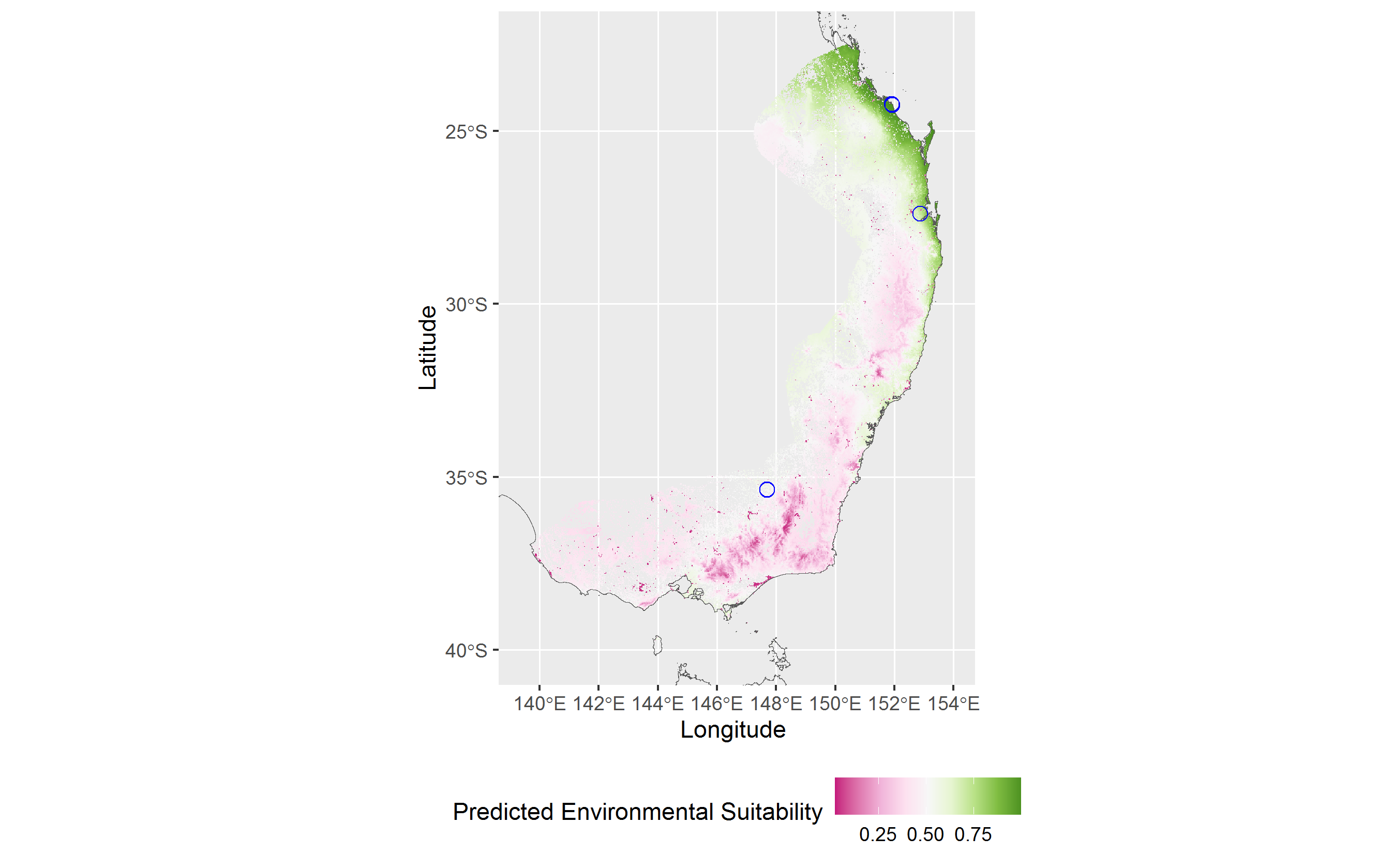
Figure 3: MaxEnt prediction of environmental suitability using Powerful Owl prescence data and five environmental layers. Prescenes are marked with blue circles (note that some records are overlapping due to the scale).
When comparing presence only data with presence / absence data, again results varied by species, but were most interesting for a species that had close to the same number of presence and absence data available, the Masked Owl. Using this owl’s presence only data in a Bioclim model resulted in a reasonable approximation of geographic distribution in southern Australia (Figure 4). However, that model completely failed to predict the presence of this owl in much of northern Australia. When presence absence data was run through a Artificial Neural Network model, the predictions included all of northern Australia (Figure 5) and were much more closely aligned to the known continental distribution of Masked Owl.
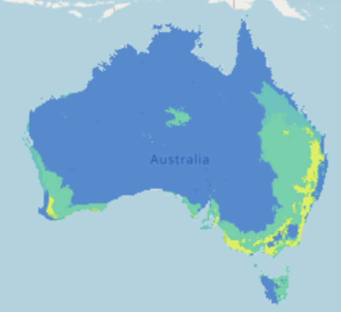
Figure 4: Masked Owl distribution prediction using a Bioclim model (presence only), generated on the EcoCommons platform.
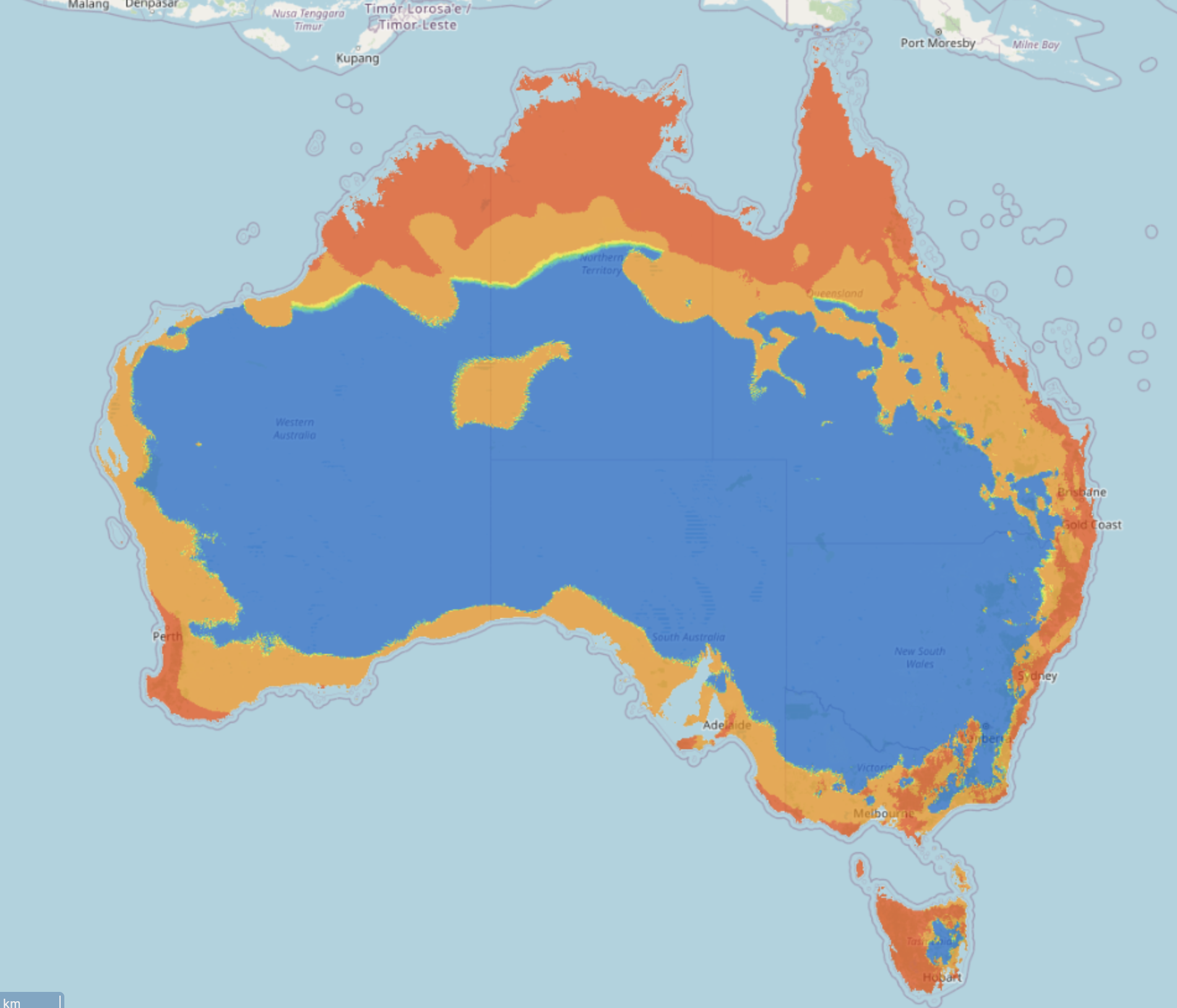
Figure 5: Masked Owl distribution prediction using a Artificial Neural Network model (presence / absence data), generated on the EcoCommons platform.
The mapped frequency of Southern Boobook suggests that it would be possible to predict areas where these owls call more (Figure 6). The results demonstrated some reasonable patterns, such as increased call frequency along what might be creeks or waterways in the outback, while the lowest call frequencies were in outback deserts. The high call frequency in SW WA also looked reasonable, but the lack of similar high call frequency areas in much of eastern Australia are likely due to insufficient sampling in this region.
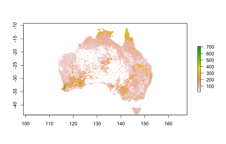
Figure 6: Predicted call frequency (number of calls) of the Southern Boobook, using a Boosted Regression Tree.
Discussion #
It was surprising how well some of the data predicted continental distributions despite there being relatively few records available (< 37 for each species). It was also striking how vastly different predictions were when using presence only vs presence absence data. Finally, the variation in predicted call frequency of the Southern Boobook across Australia suggests that the metric of call frequency may be a useful indicator of habitats that get more use, potentially related to habitat quality or breeding activity.
Initial attempts to model with 25m resolution proved to be too much data to handle, but further work to tile data extractions and predictions would likely allow such high resolution predictions, and while not useful at the continental scale modelled here, there were some stations that were fairly close together, and with fine resolution data it might be possible to tease apart the within cluster variation in presences or frequency of presences.
It is well established that acoustic monitoring can provide significant
ecological insights, across both broad spatial and temporal scales. As acoustic
monitoring activities continue to grow, we demonstrate that when such data is
annotated, whether by using
recognisers
Acknowledgements #
- We would like to first acknowledge the Australian Acoustic Observatory
(A2O)
for the recording data. - The Hoot Detective project for providing the annotations.
- We would also like to acknowledge the
EcoCommons
platform for generating some of the models used for this use case: - To learn more about Species Distribution Modelling, you can visit the
EcoCommons support page section on
SDMs
. - Visit the Educational Material
section to learn about using the EcoCommons modelling platform. - Read more about ecoacoustic integration with EcoCommons
here
.
- To learn more about Species Distribution Modelling, you can visit the
EcoCommons support page section on
SDMs